varrank: An R Package for Variable Ranking Based on Mutual Information with Applications to Systems Epidemiology
Gilles Kratzer, Reinhard Furrer
2020-01-29
varrank.RmdWhat is the package design for?
The two main problems addressed by this package are selection of the most representative variable within a group of variables of interest (i.e. dimension reduction) and variable ranking with respect to a set of features of interest.
How does it work?
The varrank R package takes a named dataset as input. It transforms the continuous variables into categorical ones using discretization rules. Then a varrank analysis sequentially compares relevance with redundancy. The final rank is based on the measure of this score.
What are the R package functionalities?
The workhorse of the R package is the varrank() function. It computes the rank of variables and it returns a varrank class object. This object can be summarized with a comprehensive verbal description or a plot.
What is the structure of this document?
We first illustrate the package with a simple example. In a second step we compare the output of the main function varrank() with alternative approaches. Then some details are provided. For a full description of the technical details we refer to the original publication (Kratzer and Furrer 2018).
Simple varrank example
The package is available through CRAN and can be installed directly in R:
Once installed, the varrank R package can be loaded using:
Let us start with a ranking example from the mlbench R package (Leisch and Dimitriadou 2005). The PimaIndiansDiabetes dataset contains 768 observations on 9 clinical variables. To run the varrank() function, one needs to choose a score function model (“battiti”, “kwak”, “peng”, “estevez”), a discretization method (see discretization for details) and an algorithm scheme (“forward”, “backward”).
For the first search, it is advised to use either “peng” (faster) or “estevez” (more reliable but much slower for large datasets) and, in case the number of variables is large (>100), restrict the “forward” search to “n.var = 100.” The progress bar will give you an idea of the remaining run time.
data(PimaIndiansDiabetes, package = "mlbench")
varrank.PimaIndiansDiabetes <- varrank(data.df = PimaIndiansDiabetes, method = "estevez", variable.important = "diabetes", discretization.method = "sturges", algorithm = "forward", scheme="mid", verbose = FALSE)

summary(varrank.PimaIndiansDiabetes)
#> Number of variables ranked: 8
#> forward search using estevez method
#> (mid scheme)
#>
#> Ordered variables (decreasing importance):
#>        glucose mass   age pedigree insulin pregnant pressure triceps
#> Scores   0.187 0.04 0.036   -0.005  -0.013   -0.008   -0.014      NA
#>
#>  ---
#>
#>  Matrix of scores:
#>          glucose   mass    age pedigree insulin pregnant pressure triceps
#> glucose    0.187
#> mass       0.092   0.04
#> age        0.085  0.021  0.036
#> pedigree   0.031  0.007 -0.005   -0.005
#> insulin    0.029 -0.041 -0.024   -0.015  -0.013
#> pregnant   0.044  0.013  0.017    -0.03  -0.016   -0.008
#> pressure   0.024 -0.009 -0.021   -0.024  -0.019   -0.015   -0.014
#> triceps    0.034  0.009 -0.046   -0.034  -0.024   -0.035    -0.02
The function varrank() returns a list with multiple entries: “names.selected” and “distance.m”. If algorithm = "forward", “names.selected” contains an ordered list of the variable names in decreasing order of importance relative to the set in “variable.important” and, for a backward search, the list is in increasing order of importance. The scheme of comparison between relevance and redundance should be set to “mid” (Mutual Information Difference) or “miq” (Mutual Information Quotient). In order to visually assess varrank() output, one can plot it:

Basically, the varrank() function sequentially compares the relevancy/redundancy balance of information across the set of variables. There is a legend containing the color code (cold blue for redundancy, hot red for relevancy) and the distribution of the scores. The columns of the triangular matrix contain the scores at each selection step. The variable selected at each step is the one with the highest score (the variables are ordered in the plot). The scores at selection can thus be read from the diagonal. A negative score indicates a redundancy final trade of information and a positive score indicates a relevancy final trade of information.
Comparison with other R packages
Caret
Here is the output of the caret R package (Kuhn et al. 2014) applied to the same PimaIndiansDiabetes dataset. caret allows one to perform a model-free variable selection search. In such a case, the importance of each predictor is evaluated individually using a filter approach.
library(caret)
#> Loading required package: lattice
#> Loading required package: ggplot2
library(e1071)
# prepare training scheme
control <- trainControl(method = "repeatedcv", number = 10, repeats = 3)
# train the model
model <- train(diabetes~., data = PimaIndiansDiabetes, method = "lvq", preProcess = "scale", trControl = control)
# estimate variable importance
importance <- varImp(model, useModel = FALSE)
# summarize importance
print(importance)
#> ROC curve variable importance
#>
#>          Importance
#> glucose       100.0
#> mass           59.8
#> age            59.6
#> pregnant       32.6
#> pedigree       27.3
#> pressure       19.4
#> triceps         6.3
#> insulin         0.0
# plot importance
plot(importance)
R Package Boruta
An alternative for variable selection is the Boruta R package (Kursa, Rudnicki, and others 2010). This compares the original attributes’ importance with the importance achieved by random, estimated using their permuted copies in the Random Forest method. The Boruta output from the analysis of the same dataset is as follows.
library(Boruta)
#> Loading required package: ranger
out.boruta <- Boruta(diabetes~., data = PimaIndiansDiabetes)
print(out.boruta)
#> Boruta performed 99 iterations in 11.8 secs.
#>  7 attributes confirmed important: age, glucose, insulin, mass,
#> pedigree and 2 more;
#>  No attributes deemed unimportant.
#>  1 tentative attributes left: pressure;
plot(out.boruta, cex.axis = 0.8, las=1)
R Package varSelRF
varSelRF (Diaz-Uriarte 2007) is a random forest-based R package that performs variable ranking. The output of the same analysis is as follows.
library(varSelRF)

rf <- randomForest(diabetes~., data = PimaIndiansDiabetes, ntree = 200, importance = TRUE)
rf.rvi <- randomVarImpsRF(xdata = PimaIndiansDiabetes[, 1:8], Class = PimaIndiansDiabetes[, 9], forest = rf, numrandom = 20, usingCluster = FALSE)
#>
#>  Obtaining random importances ....................
randomVarImpsRFplot(rf.rvi, rf, show.var.names = TRUE, cexPoint = 0.3,cex.axis=0.3)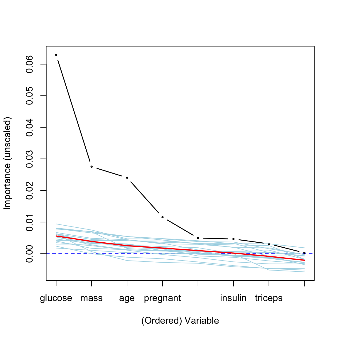
Underlying Theory of varrank
Information theory metrics
The varrank R package is based on the estimation of information theory metrics, namely, the entropy and the mututal information.
Intuitivelly, the entropy is defined as the average amount of information produced by a stochastic source of data. The mutual information is defined as the mutual dependence between the two variables.
Entropy from observational data
Formally, for a continuous random variable \(X\) with probability density function \(P(X)\) the entropy \(\text{H}(X)\) is defined as (see Cover and Thomas 2012 for details)
\[ \text{H}(X) = \textbf{E} [ - \log{P(X)} ]. \]
The entropy \(\text{H}(X)\) of a discrete random variable \(X\) is defined as (see Cover and Thomas 2012 for details) \[ \text{H}(X) = \sum^{N}_{n = 1} P(x_n) \log{P(x_n)}, \] where \(N\) is the number of states of the random variable \(X\).
The latter definition can easily be extended for an arbitrarily large set of random variables. For \(M\) random variables with \(N_1\) to \(N_M\) possible states respectively, the joint entropy is defined as \[\begin{equation} \text{H}(X_1, \dots, X_M) = \sum^{N_1}_{x_1 = 1} \dots \sum^{N_M}_{x_M = 1}P(x_1, \dots, x_M) \log{P(x_1, \dots, x_M)}. \end{equation}\]
We now illustrate the calculation of entropy for some simple cases and give the true/theoretical values, as well.
### 1D example ####
# sample from continuous uniform distribution
x1 = runif(1000)
hist(x1, xlim = c(0, 1))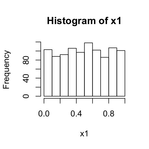
#True entropy value: H(X) = log(1000) = 6.91
entropy.data(freqs.table = table(discretization(data.df = data.frame(x1), discretization.method = "rice", freq = FALSE)))
#> [1] 4.24

# sample from a non-uniform distribution
x2 = rnorm(n = 10000, mean = 0, sd = 1)
hist(x2)
#differential entropy: H(x) = log(1*sqrt(2*pi*exp(1))) = 1.42
entropy.data(freqs.table = table(discretization(data.df = data.frame(x2), discretization.method = "sturges", freq = FALSE)))
#> [1] 2.81

### 2D example ####
# two independent random variables
x1 <- runif(100)
x2 <- runif(100)


## Theoretical entropy: 2*log(100) = 9.21
entropy.data(freqs.table = table(discretization(data.df = data.frame(x1, x2), discretization.method = "sturges", freq = FALSE)))
#> [1] 4.95
Mutual information from observational data
The mutual information \(\text{MI}(X;Y)\) of two discrete random variables \(X\) and \(Y\) is defined as (see Cover and Thomas 2012 for details) \[\begin{equation} \text{MI}(X;Y) = \sum^{N}_{n = 1} \sum^{M}_{m = 1}P(x_n,y_m) \log{\frac{P(x_ny_,m)}{P(x_n)P(y_m)} }, \end{equation}\] where \(N\) and \(M\) are the number of states of the random variables \(X\) and \(Y\), respectively. The extension to continuous variables is straightforward. The MI can also be expressed using entropy as (see Cover and Thomas 2012 for details) \[\begin{equation}\label{eq:mi_entropy} \text{MI}(X;Y) = \text{H}(X) + \text{H}(Y) -\text{H}(X, Y). \end{equation}\]
# mutual information for 2 uniform random variables
x1 <- runif(10000)
x2 <- runif(10000)

# approximately zero
mi.data(X = x1, Y = x2, discretization.method = "kmeans")
#> [1] 0.00759

# MI computed directely
mi.data(X = x2, Y = x2, discretization.method = "kmeans")
#> [1] 3.46

# MI computed with entropies:
##MI(x,y) = H(x)+H(y)-H(x, y) for x=y;
##MI(x,x) = 2 * H(x) - H(x,x)
2 * entropy.data(freqs.table = table(discretization(data.df = data.frame(x2), discretization.method = "kmeans", freq = FALSE))) - entropy.data(freqs.table = table(discretization(data.df = data.frame(x2, x2), discretization.method = "kmeans", freq = FALSE)))
#> [1] 3.46
Variables ranking/feature ranking
Mutual information is very appealing when one wants to compute the degree of dependency between multiple random variables. Indeed, as it is based on the joint and marginal probability density functions (pdfs), it is very effective in measuring any kind of relationship (Cover and Thomas 2012). The Minimum Redundancy Maximum Relevance (mRMR) algorithm can be described as an ensemble of models (Van Dijck and Van Hulle 2010), originally proposed by Battiti (1994) and coined by Peng, Long, and Ding (2005). A general formulation of the ensemble of the mRMR technique is as follows. Given a set of features \(\textbf{F}\), a subset of important features \(\textbf{C}\), a candidate feature \(f_i\) and possibly some already selected features \(f_s \in \textbf{S}\), the local score function for a scheme in difference (Mutual Information Difference) is expressed as:
\[\begin{equation} g(\alpha, \beta, \textbf{C}, \textbf{S}, \textbf{F}) = \text{MI}(f_i;\textbf{C}) - \beta \sum_{f_s \in \textbf{S}} \alpha(f_i, f_s, \textbf{C}) ~\text{MI}(f_i; f_s). \end{equation}\]
This equation is called the mRMRe equation. Model names and their corresponding functions \(\alpha\) and parameters \(\beta\) are listed below in historical order of publication:
\(\beta>0\) is a user defined parameter and \(\alpha(f_i,f_s,\textbf{C})=1\), named mutual information feature selector (MIFS). This method is called in varrank and presented in Battiti (1994).
\(\beta>0\) is a user defined parameter and \(\alpha(f_i,f_s,\textbf{C})={\text{MI}(f_s;\textbf{C})}/{\text{H}(f_s)}\), named MIFS-U. This method is called in varrank and presented in Kwak and Choi (2002).
\(\beta={1}/{|\textbf{S}|}\) and \(\alpha(f_i,f_s,\textbf{C})=1\), which is named min-redundancy max-relevance (mRMR). This method is called in varrank and presented in Peng, Long, and Ding (2005).
\(\beta={1}/{|\textbf{S}|}\) and \(\alpha(f_i,f_s,\textbf{C})={1}/{\text{min}(\text{H}(f_i),\text{H}(f_s))}\) named Normalized MIFS (NMIFS). This method is called in varrank and presented in Estévez et al. (2009).
The two terms on the right-hand side of the definition of the local score function above are local proxies for the relevance and the redundancy, respectively. Redundancy is a penalty included to avoid selecting features highly correlated with previously selected ones. Local proxies are needed because computing the joint MI between high dimensional vectors is computationally expensive. The function \(\alpha\) and the parameter \(\beta\) attempt to balance both terms to the same scale. In Peng, Long, and Ding (2005) and Estévez et al. (2009), the ratio of comparison is adaptively chosen as \(\beta = 1/{|S|}\) to control the second term, which is a cumulative sum and increases quickly as the cardinality of \(\textbf{S}\) increases. The function \(\alpha\) tends to normalize the right side. One can remark that \(0 \leq \text{MI}(f_i;f_s) \leq \min(\text{H}(f_i), \text{H}(f_s))\).
Software implementation
A common characteristic of data from systems epidemiology is that it contains both discrete and continuous variables. Thus, a common popular and efficient choice for computing information metrics is to discretize the continuous variables and then deal with only discrete variables. A recent survey of discretization techniques can be found in Garcia et al. (2013). Some static univariate unsupervised splitting approaches are implemented in the package. In the current implementation, one can give a user-defined number of bins (not recommended) or use a histogram-based approach. Popular choices for the latter are: Cencov’s rule (Cencov 1962), Freedman-Diaconis’ rule (Freedman and Diaconis 1981), Scott’s rule (Scott 2010), Sturges’ rule (Sturges 1926), Doane’s formula (Doane 1976) and Rice’s rule. The MI is estimated through entropy using mRMRe equation and the count of the empirical frequencies. This is a plug-in estimator. Another approach is to use a clustering approach with the elbow method to determine the optimal number of clusters. Finally, one very popular MI estimation compatible only with continuous variables is based on nearest neighbors (Kraskov, Stögbauer, and Grassberger 2004). The workhorse of varrank is the forward/backward implementation of mRMRe equation. The sequential forward variable ranking algorithm is described in (Kratzer and Furrer 2018).
Software functionalities
The package varrank exploits the object oriented functionalities of R through the S3 class. The function varrank() returns an object of class varrank, a list with multiple entries. At present, three S3 methods have been implemented: the print method displaying a condensed output, the summary method displaying the full output and a plot method. The plot method is an adapted version of heatmap.2() from the R package gplots.
output <- varrank(data.df = PimaIndiansDiabetes, method = "battiti", variable.important = "diabetes", discretization.method = "sturges", ratio = 0.6, algorithm = "forward", scheme="mid", verbose = FALSE)

##print
output
#> [1] "glucose"  "mass"     "pedigree" "age"      "insulin"  "pressure"
#> [7] "pregnant" "triceps"

##summary
summary(output)
#> Number of variables ranked: 8
#> forward search using battiti method
#> (mid scheme)
#>
#> Ordered variables (decreasing importance):
#>        glucose  mass pedigree    age insulin pressure pregnant triceps
#> Scores   0.187 0.046   -0.032 -0.068  -0.185   -0.268   -0.399      NA
#>
#>  ---
#>
#>  Matrix of scores:
#>          glucose   mass pedigree    age insulin pressure pregnant triceps
#> glucose    0.187
#> mass       0.092  0.046
#> pedigree   0.031  0.002   -0.032
#> age        0.085  0.008   -0.037 -0.068
#> insulin    0.029 -0.061   -0.106 -0.149  -0.185
#> pressure   0.024 -0.026   -0.111  -0.15  -0.232   -0.268
#> pregnant   0.044 -0.003   -0.037 -0.068  -0.317   -0.341   -0.399
#> triceps    0.034  0.002   -0.173 -0.212  -0.266   -0.407   -0.479
The plot display depends on whether the algorithm is run in a forward search or backward search.
output <- varrank(data.df = PimaIndiansDiabetes, method = "battiti", variable.important = "diabetes", discretization.method = "sturges", ratio = 0.6, algorithm = "forward", scheme="mid", verbose = FALSE)

plot(output)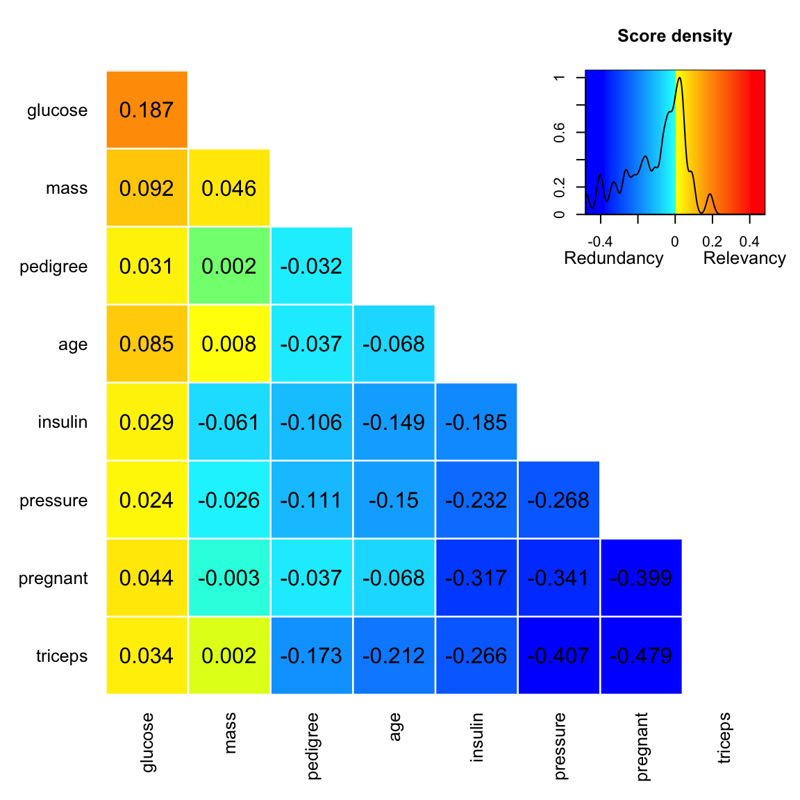
output<-varrank(data.df = PimaIndiansDiabetes, method = "battiti", variable.important = "diabetes", discretization.method = "sturges", ratio = 0.6, algorithm = "backward",scheme="mid", verbose = FALSE)

plot(output)
Examples based on different datasets
Below are some examples of the varrank methodology applied to classical R datasets.
Swiss Fertility and Socioeconomic Indicators (1888) Data
The swiss fertility dataset (R Core Team 2017) consists of six continuous variables with 47 observations.
Exploratory data analysis:

summary(lm(Fertility ~ . , data = swiss))
#>
#> Call:
#> lm(formula = Fertility ~ ., data = swiss)
#>
#> Residuals:
#>     Min      1Q  Median      3Q     Max
#> -15.274  -5.262   0.503   4.120  15.321
#>
#> Coefficients:
#>                  Estimate Std. Error t value Pr(>|t|)
#> (Intercept)       66.9152    10.7060    6.25  1.9e-07 ***
#> Agriculture       -0.1721     0.0703   -2.45   0.0187 *
#> Examination       -0.2580     0.2539   -1.02   0.3155
#> Education         -0.8709     0.1830   -4.76  2.4e-05 ***
#> Catholic           0.1041     0.0353    2.95   0.0052 **
#> Infant.Mortality   1.0770     0.3817    2.82   0.0073 **
#> ---
#> Signif. codes:  0 '***' 0.001 '**' 0.01 '*' 0.05 '.' 0.1 ' ' 1
#>
#> Residual standard error: 7.17 on 41 degrees of freedom
#> Multiple R-squared:  0.707,  Adjusted R-squared:  0.671
#> F-statistic: 19.8 on 5 and 41 DF,  p-value: 5.59e-10
Forward varrank analysis:
swiss.varrank <- varrank(data.df = swiss, method = "estevez", variable.important = "Fertility", discretization.method = "sturges", algorithm = "forward", scheme = "mid", verbose = FALSE)
swiss.varrank
#> [1] "Catholic"         "Infant.Mortality" "Education"
#> [4] "Examination"      "Agriculture"
plot(swiss.varrank)
Longley
This is a data frame with seven continuous economical variables from the US, observed yearly from 1947 to 1962. This dataset is known to be highly collinear (R Core Team 2017).
The exploratory data analysis:

summary(fm1 <- lm(Employed ~ ., data = longley))
#>
#> Call:
#> lm(formula = Employed ~ ., data = longley)
#>
#> Residuals:
#>     Min      1Q  Median      3Q     Max
#> -0.4101 -0.1577 -0.0282  0.1016  0.4554
#>
#> Coefficients:
#>               Estimate Std. Error t value Pr(>|t|)
#> (Intercept)  -3.48e+03   8.90e+02   -3.91  0.00356 **
#> GNP.deflator  1.51e-02   8.49e-02    0.18  0.86314
#> GNP          -3.58e-02   3.35e-02   -1.07  0.31268
#> Unemployed   -2.02e-02   4.88e-03   -4.14  0.00254 **
#> Armed.Forces -1.03e-02   2.14e-03   -4.82  0.00094 ***
#> Population   -5.11e-02   2.26e-01   -0.23  0.82621
#> Year          1.83e+00   4.55e-01    4.02  0.00304 **
#> ---
#> Signif. codes:  0 '***' 0.001 '**' 0.01 '*' 0.05 '.' 0.1 ' ' 1
#>
#> Residual standard error: 0.305 on 9 degrees of freedom
#> Multiple R-squared:  0.995,  Adjusted R-squared:  0.992
#> F-statistic:  330 on 6 and 9 DF,  p-value: 4.98e-10
Forward varrank analysis:
longley.varrank <- varrank(data.df = longley, method = "estevez", variable.important = "Employed", discretization.method = "sturges", algorithm = "forward", scheme = "mid", verbose = FALSE)
longley.varrank
#> [1] "GNP"          "Armed.Forces" "Population"   "GNP.deflator"
#> [5] "Year"         "Unemployed"
plot(longley.varrank)
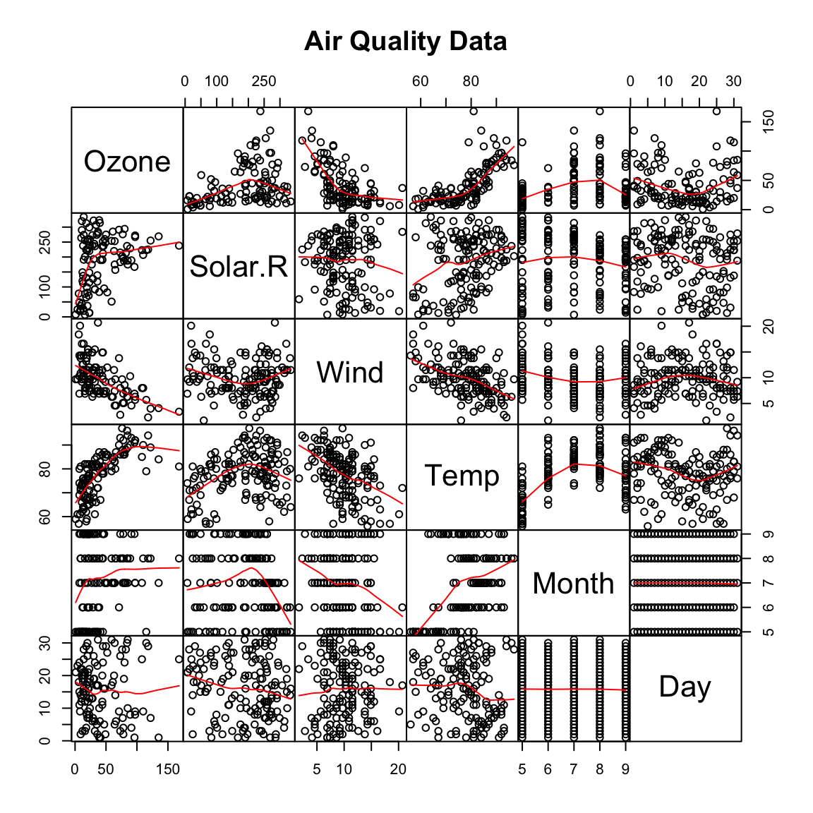
Air Quality dataset
Daily air quality measurements in New York from May to September 1973. This dataset (R Core Team 2017) contains 6 continuous variables with 154 observations. A complete case analysis is performed.
Exploratory data analysis:
Forward varrank analysis
airquality.varrank <- varrank(data.df = (data.frame(lapply(airquality[complete.cases(airquality), ], as.numeric))), method = "estevez", variable.important = "Ozone", discretization.method = "sturges", algorithm = "forward", scheme = "mid", verbose = FALSE)
airquality.varrank
#> [1] "Temp"    "Wind"    "Day"     "Solar.R" "Month"
plot(airquality.varrank)
Airbags and other influences on accident fatalities
This is US data (1997-2002) from police-reported car crashes in which there was a harmful event (people or property) and from which at least one vehicle was towed. This dataset (Maindonald and Braun 2014) contains 15 variables with 26’217 observations. The varrank forward search is performed using “peng” model.
data(nassCDS)

nassCDS.varrank <- varrank(data.df = nassCDS, method = "peng", variable.important = "dead", discretization.method = "sturges", algorithm = "forward", scheme = "mid", verbose = FALSE)
nassCDS.varrank
#>  [1] "injSeverity" "frontal"     "ageOFocc"    "yearacc"     "dvcat"
#>  [6] "occRole"     "weight"      "seatbelt"    "sex"         "airbag"
#> [11] "deploy"      "yearVeh"     "abcat"       "caseid"

plot(nassCDS.varrank, notecex = 0.5)
Bibliography
Battiti, Roberto. 1994. “Using Mutual Information for Selecting Features in Supervised Neural Net Learning.” IEEE Transactions on Neural Networks 5 (4). IEEE: 537–50.
Cencov, NN. 1962. “Estimation of an Unknown Density Function from Observations.” In Dokl. Akad. Nauk, Sssr, 147:45–48.
Cover, Thomas M, and Joy A Thomas. 2012. Elements of Information Theory. John Wiley & Sons.
Diaz-Uriarte, Ramón. 2007. “GeneSrF and varSelRF: A Web-Based Tool and R Package for Gene Selection and Classification Using Random Forest.” BMC Bioinformatics 8 (1). BioMed Central: 328. https://CRAN.R-project.org/package=varSelRF.
Doane, David P. 1976. “Aesthetic Frequency Classifications.” The American Statistician 30 (4). Taylor & Francis Group: 181–83.
Estévez, Pablo A, Michel Tesmer, Claudio A Perez, and Jacek M Zurada. 2009. “Normalized Mutual Information Feature Selection.” IEEE Transactions on Neural Networks 20 (2). IEEE: 189–201.
Freedman, David, and Persi Diaconis. 1981. “On the Histogram as a Density Estimator: L 2 Theory.” Zeitschrift für Wahrscheinlichkeitstheorie und verwandte Gebiete 57 (4). Springer: 453–76.
Garcia, Salvador, Julian Luengo, José Antonio Sáez, Victoria Lopez, and Francisco Herrera. 2013. “A Survey of Discretization Techniques: Taxonomy and Empirical Analysis in Supervised Learning.” IEEE Transactions on Knowledge and Data Engineering 25 (4). IEEE: 734–50.
Kraskov, Alexander, Harald Stögbauer, and Peter Grassberger. 2004. “Estimating Mutual Information.” Physical Review E 69 (6). APS: 066138.
Kratzer, Gilles, and Reinhard Furrer. 2018. “Varrank: An R Package for Variable Ranking Based on Mutual Information with Applications to Observed Systemic Datasets.” arXiv.
Kuhn, M, Jed Wing, Stew Weston, Andre Williams, Chris Keefer, Allan Engelhardt, Tony Cooper, et al. 2014. Caret: Classification and Regression Training. https://CRAN.R-project.org/package=caret.
Kursa, Miron B, Witold R Rudnicki, and others. 2010. “Feature Selection with the Boruta Package.” Journal of Statistical Software 36 (11): 1–13. https://CRAN.R-project.org/package=Boruta.
Kwak, Nojun, and Chong-Ho Choi. 2002. “Input Feature Selection for Classification Problems.” IEEE Transactions on Neural Networks 13 (1). IEEE: 143–59.
Leisch, Friedrich, and Evgenia Dimitriadou. 2005. “Mlbench: Machine Learning Benchmark Problems,” 1–0. https://CRAN.R-project.org/package=mlbench.
Maindonald, John, and W John Braun. 2014. “DAAG: Data Analysis and Graphics Data and Functions. R Package Version 1.20.” https://CRAN.R-project.org/package=DAAG.
Peng, Hanchuan, Fuhui Long, and Chris Ding. 2005. “Feature Selection Based on Mutual Information Criteria of Max-Dependency, Max-Relevance, and Min-Redundancy.” IEEE Transactions on Pattern Analysis and Machine Intelligence 27 (8). IEEE: 1226–38.
R Core Team. 2017. R: A Language and Environment for Statistical Computing. Vienna, Austria: R Foundation for Statistical Computing. https://www.R-project.org/.
Romanski, Piotr. 2016. “Fselector: Selecting Attributes. 2009.” R Package Version 0.18 30. https://CRAN.R-project.org/package=FSelector.
Scott, David W. 2010. “Scott’s Rule.” Wiley Interdisciplinary Reviews: Computational Statistics 2 (4). Wiley Online Library: 497–502.
Sturges, Herbert A. 1926. “The Choice of a Class Interval.” Journal of the American Statistical Association 21 (153). Taylor & Francis: 65–66. https://doi.org/10.1080/01621459.1926.10502161.
Van Dijck, Gert, and Marc M Van Hulle. 2010. “Increasing and Decreasing Returns and Losses in Mutual Information Feature Subset Selection.” Entropy 12 (10). Molecular Diversity Preservation International: 2144–70.